Convolutional Neural Networks (CNNs) are a core technology in modern computer vision, enabling tasks such as image classification, object detection, medical imaging, and autonomous driving. Beyond convolutional layers, pooling layers are also essential, helping networks learn and recognize patterns more efficiently.
Pooling acts as a form of data reduction. After convolutions generate detailed feature maps, pooling downsamples them into a more compact representation. This allows the model to retain the most relevant patterns—such as edges, textures, or shapes—while discarding less important details. As a result, training becomes more efficient, overfitting is reduced, and the network gains robustness to small shifts or scale changes in the input image.
The Pooling Process: Step-by-Step
Imagine you have a 4×4 Input Image (a grid of 16 numbers). We will use a 2×2 Filter with a Stride of 2 (meaning the window jumps 2 pixels at a time so it never overlaps). In the context of the pooling process, Stride is the «step» or the number of pixels the window (filter) moves as it slides across the image.
When we say a Stride of 2 means the window «never overlaps,» here is the visual breakdown of what is happening:
1. The Concept of Stride
Imagine you are reading a book.
-
Stride 1: You read every single word, one by one.
-
Stride 2: You skip every other word.
In Pooling, the window (the 2×2 square) «jumps» a specific distance before it stops to look at the next set of pixels.
2. Why it «Never Overlaps»
If your window is 2 pixels wide and your Stride is 2, the movement looks like this:
-
Step 1: The window covers Pixels 1 and 2.
-
The Jump: It moves 2 pixels to the right.
-
Step 2: The window now covers Pixels 3 and 4.
Because the «Jump» (2) is the same size as the «Window» (2), the second window starts exactly where the first one ended. They do not share any pixels.
3. Visual Comparison (Example)
Imagine a row of 4 pixels: [ A ] [ B ] [ C ] [ D ]
With Stride 1 (Overlapping):
-
First window sees:
[ A ] [ B ] -
Moves 1 pixel…
-
Second window sees:
[ B ] [ C ]
Result: Pixel B was processed twice! They overlap.
With Stride 2 (Non-overlapping):
-
First window sees:
[ A ] [ B ] -
Moves 2 pixels…
-
Second window sees:
[ C ] [ D ]
Result: No pixel is seen twice. They are perfectly separate.
Why is this important for your study?
-
Size Reduction: When the Stride is 2, you are essentially cutting the width and height of the image in half. A image becomes a image.
-
Efficiency: By not overlapping, the computer processes fewer windows, which makes the AI much faster.
2×2 Filter with a Stride of 2
| Col 1 | Col 2 | Col 3 | Col 4 | |
| Row 1 | 10 | 20 | 1 | 5 |
| Row 2 | 30 | 40 | 2 | 8 |
| Row 3 | 5 | 10 | 50 | 60 |
| Row 4 | 2 | 4 | 70 | 80 |
2. Max Pooling (Extracting the «Peak»)
The filter looks at each 2×2 block and picks the highest number.
-
Top-Left Block: {10, 20, 30, 40} Max is 40.
-
Top-Right Block: {1, 5, 2, 8} Max is 8.
-
Bottom-Left Block: {10, 5, 2, 4} Max is 10.
-
Bottom-Right Block: {50, 60, 70, 80} Max is 80.
The Result (Output):
| 40 | 8 |
| 10 | 80 |
Why? It keeps the most prominent features (like a bright pixel or a sharp edge).
3. Average Pooling (Calculating the «Smoothness»)
The filter looks at the same 2×2 blocks but calculates the mean (sum divided by 4).
-
Top-Left Block:
-
Top-Right Block:
-
Bottom-Left Block:
-
Bottom-Right Block:
The Result (Output):
| 25 | 4 |
| 5.25 | 65 |
Why? It provides a smoother summary of the area.
-
If stride = 1, the filter moves 1 pixel at a time.
-
If stride = 2, it moves 2 pixels at a time.
-
If stride = 3, it moves 3 pixels at a time.

© Image. https://www.digitalocean.com/
Why Does Stride Change the Output Size?
When the filter moves with bigger steps, it looks at fewer positions in the image.
That means:
-
Stride = 1 → Output image is almost the same size
-
Stride = 2 → Output image is about half the size
-
Stride = 3 → Output image is about one third the size
So when stride > 1, the output becomes smaller.
What About Pooling?
In pooling layers:
-
The stride is usually the same as the filter size by default.
For example:
-
If the filter size is (2 × 2)
-
The stride is usually 2
This means the filter moves without overlapping.
Types of Pooling
-
Max Pooling → Keeps the biggest value in each small region
-
Average Pooling → Takes the average value in each small region

© Image. https://www.digitalocean.com/

© Image. https://www.digitalocean.com/
Why Do We Use Pooling?
To Reduce Size
Pooling reduces the width and height of the image.
This is called down-sampling.
Example:
-
A 400×400 image
-
After pooling several times
-
It could become 25×25
But it still keeps the main shape and structure.
To Make the Model Faster
Smaller images = less data
Less data = faster training and less computation
This helps the neural network work efficiently.
To Make the Model More Robust
Pooling helps the network recognize objects even if they move slightly in the image.
For example:
-
A car on the left
-
A car on the right
The network can still recognize it as a car.
This is called translation invariance.
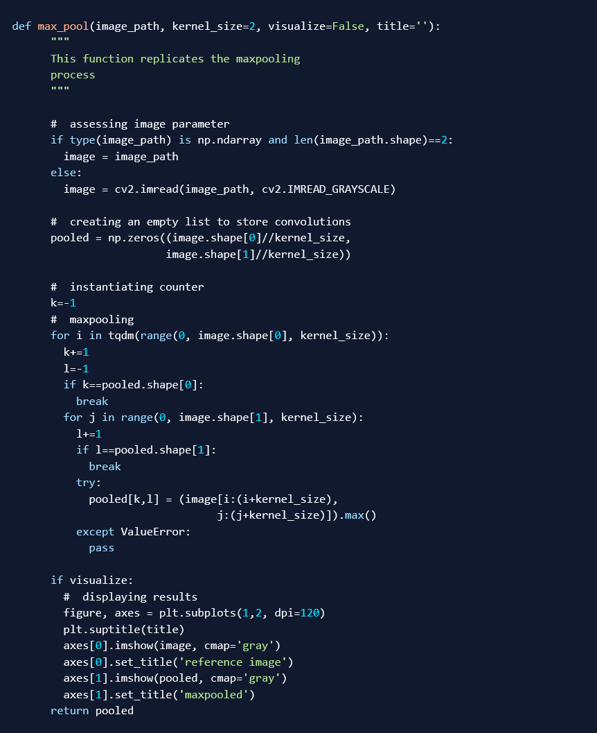
Max Pooling Function
© Image. https://www.digitalocean.com/
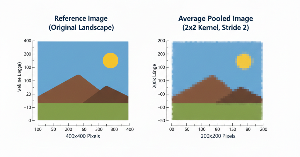
In this section, we will use manually written pooling functions to visualize the pooling process and better understand what actually goes on. Two functions are provided, one for max pooling and the other for average pooling. Using the functions, we will attempt to pool the image.
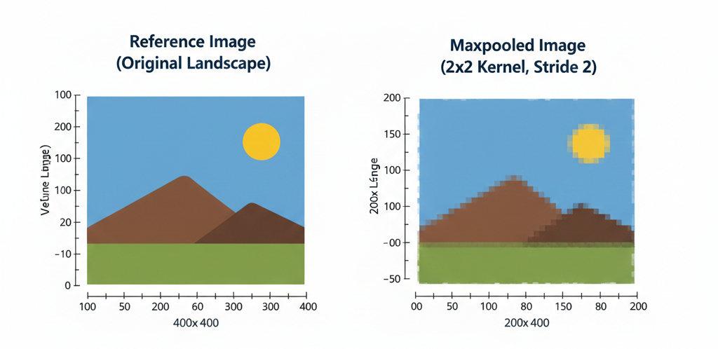
The function above replicates the max pooling process. Using the function, let’s attempt to max pool the reference image using a (2, 2) kernel.
max_pool(‘image.jpg’, 2, visualize=True)
The effects of using a larger kernel (3, 3) are seen below. As expected, the reference image reduces to 1/3 its preceding size for every iteration. By the third iteration, a pixelated (16, 16) down-sampled representation is produced (a 0.1% summary). Although pixelated, the overall idea of the image is somewhat still maintained.
visualize_pooling('image.jpg', 3, kernel=3)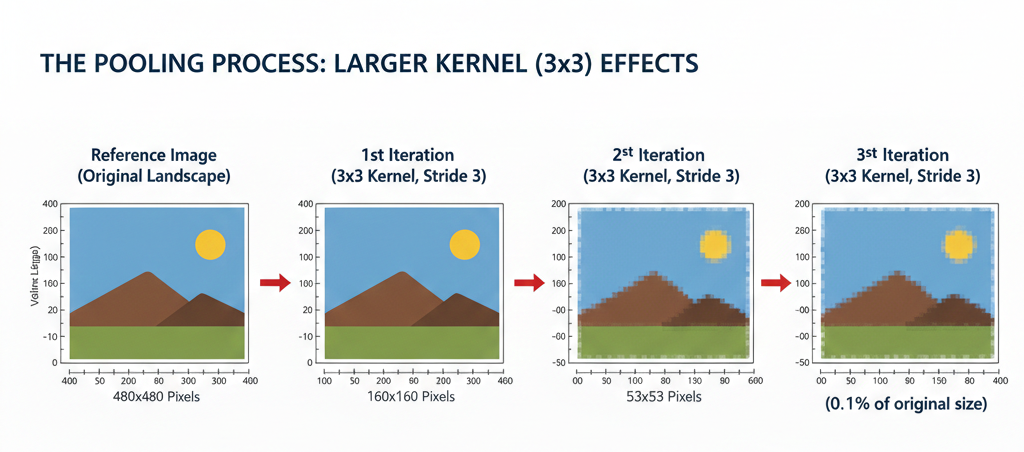
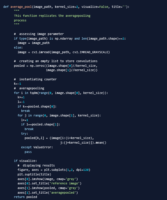
Average pooling function
© Image. https://www.digitalocean.com/
Applying Max Pooling and Average Pooling in Architecture and Construction
Pooling techniques such as max pooling and average pooling can be very useful in the architecture and construction sector, especially when using computer vision systems for inspection, monitoring, and analysis.
Applications with Large-Scale Image Data
When working with massive image datasets, pooling becomes especially valuable because it reduces dimensionality while preserving meaningful patterns.
Digital Twins and BIM Integration
In large infrastructure projects, thousands of images are generated from:
-
Site scans
-
Drones
-
3D reconstruction workflows
Pooling helps compress visual information before integrating it into digital twins or BIM-based monitoring systems, enabling scalable updates without overwhelming computational resources.
Material and Surface Classification
In large construction databases, pooling enables efficient classification of:
-
Concrete types
-
Façade materials
-
Roofing systems
-
Pavement conditions…
Reducing resolution while keeping dominant features improves scalability when processing millions of images.
Key Insight
Whenever image datasets become large — spatially (high resolution), temporally (continuous monitoring), or geographically (urban scale) — pooling is essential.
It enables models to scale from single-building analysis to city-level intelligence without prohibitive computational cost.
 @Yolanda Muriel
