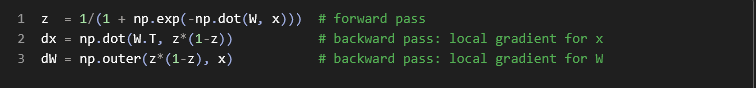
In early neural networks, it was common to use sigmoid or tanh activation functions in fully connected layers. The subtle problem is that these activations can easily saturate if your weight initialization or data preprocessing is poorly chosen.
When a sigmoid saturates, its output becomes very close to 0 or 1. In those regions, the derivative of the sigmoid is almost zero. During backpropagation this means the gradients disappear, so the network stops learning completely. Your training loss becomes flat and refuses to decrease.
The objects
- x: the input column vector (a list of numbers stacked vertically). Shape: (n,) or (n×1).
- W: the weight matrix that multiplies x. Shape: (m×n) (m neurons, n inputs).
- z: the output of applying the sigmoid activation to the linear combination
W x. Shape: (m,).
z (each between 0 and 1).In backpropagation, we need derivatives. For the sigmoid, the derivative is σ(u)·(1−σ(u)). Since z = σ(u), the derivative is z*(1-z).
W.T is the transpose of W (rows/columns swapped).
Multiplying W.T by z*(1-z) gives how changes in x would change the output (the local gradient wrt x).
np.outer(a, b) creates a matrix where each element is a_i * b_j.
Here, a = z*(1-z) (the sigmoid derivative per neuron) and b = x (each input value).
The result is an (m×n) matrix: for each neuron (m rows) and each input feature (n columns), it tells how much changing that weight would change the output—the local gradient of the output w.r.t. each weight.
- Forward: compute outputs z = sigmoid(Wx).
- Backward (w.r.t. inputs): dx = Wᵀ · (z·(1−z)) says how changes in inputs would affect outputs after the sigmoid.
- Backward (w.r.t. weights): dW = outer(z·(1−z), x) says how each weight affects the outputs and how it should be updated.

The derivative of the sigmoid—its local gradient—is:
In other words: a sigmoid can never pass a gradient bigger than 0.25.
So every time a gradient flows backward through a sigmoid, the signal is reduced to one quarter of its original size (or even smaller, if z is not exactly 0.5).
If your network has multiple sigmoid layers stacked, this repeated shrinking makes the lower layers receive extremely tiny gradients.
If you are training with plain stochastic gradient descent (SGD), this means:
- the top layers (near the output) get decent gradients and learn faster
- the bottom layers (near the input) get very small gradients and learn painfully slowly
This is one of the classic reasons that deep networks were hard to train before the introduction of ReLU and better initialization techniques.
References
© Images. https://cs231n.github.io/
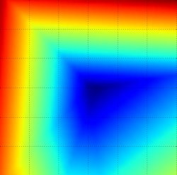
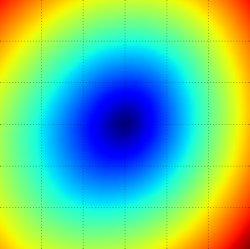
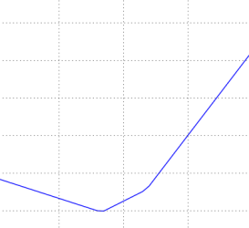
Loss function landscape for the Multiclass SVM (without regularization) for one single example (left,middle) and for a hundred examples (right) in CIFAR-10. Left: one-dimensional loss by only varying a. Middle, Right: two-dimensional loss slice, Blue = low loss, Red = high loss. Notice the piecewise-linear structure of the loss function. The losses for multiple examples are combined with average, so the bowl shape on the right is the average of many piece-wise linear bowls (such as the one in the middle).
 @Yolanda Muriel
