Before working with deep learning models, we need to import the tools that will support numerical computation, optimization, and visualization. If you come from engineering or architecture rather than computer science, think of this step as preparing the calculation environment before running a simulation or structural analysis.

Below is a breakdown of the imports commonly used in a PyTorch deep learning lab. But first a little introduction of meanings:

In any neural network:

• You have inputs

• You apply operations (linear layers, activations, etc.)

• You get an output

• You compute a loss

• You adjust parameters using derivatives

The key point: training = computing derivatives efficiently

PyTorch’s autograd package is the engine that does this for you.

autograd: automatic differentiation (why it matters)

"autograd provides automatic differentiation for all operations on Tensors.”

This means:

• Every time you perform an operation on a PyTorch Tensor

• PyTorch records that operation

• Later, it can compute exact derivatives automatically

You do NOT:

• Derive formulas by hand

• Implement backprop yourself

• Worry about the chain rule explicitly

From an engineering perspective:
This is like having a symbolic + numeric differentiation engine embedded in your code.

“Define-by-run” (dynamic behavior)

“It is a define-by-run framework”

This is extremely important.

Define-by-run means:

• The computational graph is built as your code executes

• Not beforehand

• Every iteration can be different

Contrast this with older frameworks:

• You first defined a static graph

• Then you ran it many times

• Same structure every iteration

In PyTorch:

if condition:
do_this()
else:
do_that()

Both branches are valid

The graph adapts dynamically

Engineering analogy:

Think of:

• A fixed circuit diagram (static graph)
  vs

• A reconfigurable system that changes topology depending on conditions

This is huge for:

• Control systems

• Adaptive models

• Simulation-based learning

“Every iteration can be different” — why this is powerful

“every single iteration can be different”

This means:

• You can change the architecture

• Change data flow

• Add/remove operations dynamically

Examples:

• Variable-length signals

• Time-dependent systems

• Physics-informed models with conditional logic

In engineering terms:
You’re not locked into a rigid mathematical pipeline.

Pytorch is a numerical simulation environment that automatically computes derivatives of everything you do.

The meaning of the following code we need use is:

Core PyTorch import

This is the heart of PyTorch.

What torch gives you:

• Tensors (like NumPy arrays, but smarter)

• GPU acceleration

• Automatic differentiation (via autograd)

Think of torch as:

NumPy + linear algebra + calculus + GPU support

Engineering analogy

Equivalent to importing:

• A numerical computation engine

• With built-in differentiation

• And hardware acceleration

Neural network module

This module contains:

• Layers (Linear, Conv2d, etc.)

• Loss functions

• Model-building utilities

You usually subclass:

Engineering view

This is a high-level abstraction layer:

• You define systems as blocks

• Each block has parameters

• Each block is differentiable

Very similar to:

• Block diagrams

• Modular system modeling

Functional API

This provides:

• Stateless operations (e.g. relu, softmax)

• No internal parameters

Example:

vs

Why both exist?

• nn → stateful modules

• F → pure functions

Engineering analogy

• nn: components with internal state

• F: pure mathematical operators

Optimizers

This is for parameter updates:

• SGD

• Adam

• RMSProp

Example:

Engineering analogy

This is your optimization algorithm:

• Gradient descent

• Numerical minimization

• Control law for parameter tuning

NumPy

Classic numerical library.

Used for:

• Data generation

• Preprocessing

• Interfacing with non-PyTorch code

Important rule:

NumPy does not track gradients
PyTorch does

So gradients stop when you convert to NumPy.

Matplotlib

This is just for:

• Plotting losses

• Visualizing results

• Debugging

%matplotlib inline:

• Jupyter magic

• Plots appear inside the notebook

Nothing to do with learning or gradients.

Timer

Used to:

• Measure execution time

• Compare CPU vs GPU

• Benchmark operations

Engineering angle

Performance matters:

• Training speed

• Algorithm efficiency

• Scalability

Automatic Differentiation in PyTorch: Understanding requires_grad and the Dynamic Computational Graph

One of the key ideas behind PyTorch — and modern deep learning in general — is automatic differentiation. If you come from engineering or architecture, you can think of this as an automated way of computing sensitivities: how a change in one variable affects the final result of a system.

PyTorch implements this mechanism through tensors, gradients, and something called a dynamic computational graph.

Tensors That Track Derivatives: requires_grad

In PyTorch, numerical data is stored in objects called Tensors.
A tensor can optionally track how it was created, meaning it can later compute derivatives.

This behavior is controlled by the attribute:

requires_grad = True

When a tensor has requires_grad=True:

• PyTorch records every operation applied to it

• These operations are stored internally

• PyTorch becomes able to compute exact gradients automatically

In practical terms:

You tell PyTorch: “This variable matters for optimization. Track how it influences the result.”

Engineering analogy

This is equivalent to:

• Marking a design parameter as optimizable

• Asking: How does changing this parameter affect cost, stress, energy consumption, or performance?

Computing Gradients Automatically: .backward()

Once all computations are done (for example, once you compute a loss or error), you call:

This triggers backpropagation.

What PyTorch does internally:

• Traverses all recorded operations backwards

• Applies the chain rule

• Computes derivatives automatically

• Stores them in the .grad attribute of each relevant tensor

So after calling .backward():

contains the gradient of the final result with respect to that tensor.

Important Detail: Gradients Are Accumulated

A critical point that often confuses beginners:

Gradients in PyTorch are accumulated, not overwritten.

This means:

• Every call to .backward() adds new gradients

• If .grad already contains values, PyTorch sums the new ones

This is intentional and useful for:

• Mini-batch training

• Iterative optimization

Engineering analogy

Think of it like:

• Accumulating load effects

• Summing sensitivities across multiple simulations

• Integrating incremental contributions over time

This is why gradients are often reset manually during training loops.

Operations Create a Computational Graph

Every mathematical operation performed on a tensor is internally represented as a node in a graph.

More precisely:

• Each operation corresponds to a Function (torch.autograd.Function)

• The result of an operation is a new tensor

• That tensor stores:

  • Where it came from

  • Which operation created it

This graph is:

• Acyclic (no loops)

• Built dynamically as the code runs

Each tensor has an attribute:

This attribute points to the function that created the tensor.

That is all the graph is:

Tensors connected by the operations that produced them.

Example: Multiplication of Two Tensors

If you multiply two tensors:

PyTorch internally records:

• The source tensors (x and y)

• The multiplication operation

• The resulting tensor (z)

This creates a small graph.

You do not need to build this graph manually.
PyTorch constructs it automatically, step by step, as your code executes.

The Dynamic Computational Graph (DCG)

This entire structure is called the Dynamic Computational Graph (DCG).

“Dynamic” means:

• The graph is built at runtime

• It reflects exactly the operations executed

• It can change between iterations

This is fundamentally different from static mathematical pipelines.

Engineering perspective

Think of the DCG as:

• A live system diagram

• Generated automatically from your calculations

• Updated every time the workflow changes

This is extremely powerful for engineering applications involving:

• Conditional logic

• Variable geometries

• Adaptive systems

• Physics-informed models

Why This Matters for the Construction and Engineering Sector

In engineering and architecture, many problems rely on:

• Optimization

• Sensitivity analysis

• Parametric design

• Performance-driven decision making

PyTorch’s automatic differentiation allows you to:

• Define complex mathematical models

• Combine physical equations with data

• Compute gradients without deriving equations manually

In other words:

You focus on modeling the system.
PyTorch handles the calculus.

Example multiplication of two tensors and the resulting interconnection.

Step 1: Two Independent Tensors

We start with two tensors:

• Tensor X, with a numerical value of 1.0

• Tensor Y, with a numerical value of 2.0

Both tensors have:

• requires_grad = False

• No stored gradient

• No associated gradient function

This means they are treated as constant inputs. PyTorch does not need to know how changes in these values affect the result, because they are not meant to be optimized.

Engineering analogy

Think of these tensors as fixed parameters:

• Known material properties

• Prescribed loads

• Constant geometric dimensions

They participate in the calculation, but we are not interested in adjusting them.

Step 2: Applying a Mathematical Operation

Next, we multiply the two tensors:

Numerically, this gives:

At this moment, PyTorch does something important behind the scenes:

• It creates a new tensor to store the result

• It records which operation produced it

• It stores references to the input tensors involved

This operation becomes a node in PyTorch’s internal computational structure.

Step 3: The Resulting Tensor

The output tensor Z has:

• data = 2.0

• requires_grad = True

• grad = None (for now)

• grad_fn = <Mul>

This tells us that:

• The tensor was produced by a multiplication

• PyTorch knows how to compute derivatives through this operation

• Gradients can be propagated backwards if needed

Why does requires_grad matter here?

Even though X and Y do not track gradients, Z does.
This allows Z to act as a connection point in a larger model, where later operations may depend on it.

Step 4: The Computational Structure That Is Created

The multiplication creates a simple chain:

• Two input tensors

• One mathematical operation (multiplication)

• One output tensor

This structure is part of what PyTorch calls a dynamic computational graph.

Key characteristics:

• Built automatically

• Built during execution

• Exists only for the current computation

• Fully describes how the result was obtained

You do not draw this graph.
You do not define it manually.
PyTorch reconstructs it every time your code runs.

Python code: creating tensors, operating on them, and computing derivatives

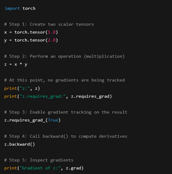
import torch

# Step 1: Create two scalar tensors
x = torch.tensor(1.0)
y = torch.tensor(2.0)

# Step 2: Perform an operation (multiplication)
z = x * y

# At this point, no gradients are being tracked
print(«z:», z)
print(«z.requires_grad:», z.requires_grad)

# Step 3: Enable gradient tracking on the result
z.requires_grad_(True)

# Step 4: Call backward() to compute derivatives
z.backward()

# Step 5: Inspect gradients
print(«Gradient of z:», z.grad)

What is happening step by step

Creating the tensors

We start with two scalar tensors (x and y).
They represent simple numerical values and do not track gradients.

This means:

• PyTorch performs the multiplication

• But no derivative information is stored yet

Creating a Dynamic Computational Graph

When we compute:

PyTorch builds a dynamic computational graph describing:

• Which tensors were involved

• Which operation was applied

However, none of the nodes require gradients, so the graph is incomplete from an optimization perspective.

Enabling gradient tracking

By calling:

we tell PyTorch:

“This value is important. I want to know how it behaves when backpropagating.”

Now z becomes a valid starting point for differentiation.

Calling the life saver: backward()

When we run:

PyTorch:

• Traverses the graph backwards

• Applies the chain rule

• Computes the derivative of z with respect to itself

Since z is a scalar, the result is:

That is why:

Engineering intuition

This is equivalent to:

• Defining a calculation

• Declaring which result matters

• Asking: “How does this result change?”

Even though this is a minimal example, the exact same mechanism applies to:

• Large systems

• Complex equations

• Deep neural networks

• Engineering optimization problems

First example of python code is: a case that crashes on purpose. Following we have an example that:

• Know the correct way to enable gradient tracking

• Show the change in the Tensor description

• Highligh requires_grad and grad_fn = MulBackward

import torch

# ———————————-
# 1. This WILL crash (intentionally)
# ———————————-

x = torch.tensor(1.0)
y = torch.tensor(2.0)

z = x * y

print(«z.requires_grad:», z.requires_grad)

# This will raise an error because no tensor tracks gradients
try:
z.backward()
except RuntimeError as e:
print(«Expected crash:»)
print(e)

# ———————————-
# 2. Correct approach: enable gradients
# ———————————-

x = torch.tensor(1.0, requires_grad=True)
y = torch.tensor(2.0, requires_grad=True)

z = x * y

# Inspect the tensor
print(«\nNew z tensor:»)
print(«z:», z)
print(«z.requires_grad:», z.requires_grad)
print(«z.grad_fn:», z.grad_fn)

# ———————————-
# 3. Call backward successfully
# ———————————-

z.backward()

# Inspect gradients
print(«\nGradients after backward():»)
print(«dz/dx =», x.grad)
print(«dz/dy =», y.grad)

What this code demonstrates (conceptually)

First case: why it crashes

In the first block:

• Neither x nor y has requires_grad=True

• PyTorch builds the numerical result

• No gradient graph is created

• Calling backward() is meaningless → crash is expected

This is intentional behavior, not a bug.

Second case: enabling gradient tracking correctly

Here we enable gradient tracking at tensor creation time:

Now:

• PyTorch tracks all operations

• The multiplication produces a tensor z

• z automatically:

  • Requires gradients

  • Stores a reference to its origin operation

The key difference: grad_fn

When you inspect:

You will see something like:

This means:

• z was created by a multiplication

• PyTorch knows how to compute its derivative

• During backward(), this operation will be differentiated

This is the proof that:

The multiplication is part of the computational graph
and will participate in backpropagation.

Conclusion: Why This Matters for Architecture, Engineering, and Construction

At first glance, automatic differentiation may appear to be a purely academic or machine-learning-specific concept. However, when viewed through the lens of the AEC sector, its relevance becomes immediately clear.

In architecture and engineering, we routinely work with systems where outcomes depend on many interrelated parameters: geometry, materials, loads, energy flows, costs, and constraints. Traditionally, understanding how a small change in one parameter affects the overall system requires either simplified assumptions or manual sensitivity analysis.

PyTorch’s dynamic computational graph and automatic differentiation fundamentally change this workflow. Instead of deriving gradients by hand or approximating them numerically, engineers can define their models directly — using equations, rules, and conditional logic — and let the framework compute exact sensitivities automatically.

This capability opens the door to:

• Gradient-based optimization of designs and systems.

• Data-driven performance models integrated with physics.

• Parametric exploration at scales that were previously impractical.

• New ways of combining simulation, data, and optimization.

Most importantly, deep learning tools like PyTorch are not limited to neural networks. They are general-purpose engines for differentiable computation. For the AEC sector, this means that deep learning is not just about prediction — it is about better decision-making, better optimization, and more intelligent design workflows.

Understanding these foundations is the first step toward applying artificial intelligence meaningfully and responsibly in the built environment.

@Yolanda Muriel Attribution-NonCommercial-NoDerivs 3.0 Unported (CC BY-NC-ND 3.0)