On the article ARTIFICIAL INTELLIGENCE (29) – Deep learning (18) – Monitoring Deep Learning Models with TensorBoard: Reconstruction and Classification on MNIST We explore how to monitor machine learning models using TensorBoard, focusing on two fundamental deep learning tasks:
- Image reconstruction using an autoencoder
- Digit classification using a simple neural network
In this article we explore how to monitor machine learning models using BandB, focusing on two fundamental deep learning tasks:
- Image reconstruction using an autoencoder
- Digit classification using a simple neural network
Logging MNIST Reconstruction ; Classification with WandB. WandB (Weights & Biases) is similar to TensorBoard but offers:
-automatic dashboards
-online logging
-image galleries
-confusion matrices
-system metrics
-hyperparameter tracking
-experiment comparison
-report creation
It is cloud‑based and much easier to use than TensorBoard.
Step 1 — Create a WandB account
1. Go to:
https://wandb.ai
2. Sign in with:
Google, or
GitHub, or
Email
Environment Setup and Execution
We created a Python virtual environment, installed required dependencies, and executed the two experiments with the following commands:
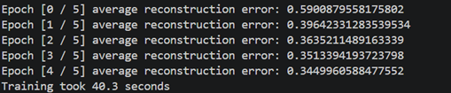
Reconstruction task
python main.py –task reconstruction –log_framework wandb
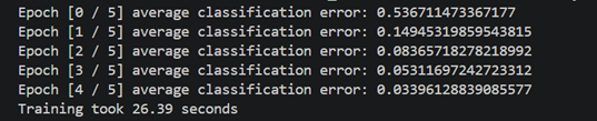
python main.py –task classification –log_framework wandb
WandB Reconstruction Visual Analysis
WandB run produced several reconstructed image grids. These grids show how the autoencoder learns to compress and reconstruct MNIST digits over the training epochs.
Each grid typically contains:
- The original input images.
- The reconstructed images at different stages of training.
- Sometimes noise-only grids (when the model has not yet learned meaningful features).
I will describe the purpose and interpretation of each of the images.
Image 1 — Original MNIST Batch
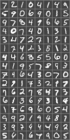
This grid shows a batch of original MNIST digits. It is the reference the autoencoder uses to learn.
Interpretation
- Clear, human‑readable digits.
- Includes all digits 0–9 distributed randomly.
- This is used to compare visually against the reconstructions below.
This is the baseline: what the model tries to reconstruct.
Image 2 — Noise Output (Untrained or Bad Decoder Init)
This grid contains pure noise, not digits.
Interpretation
This happens when:
- the reconstruction is captured before any training steps,
or - the logged batch corresponds to random decoder output before learning begins.
This is normal.
Early in training, the autoencoder has no idea how MNIST digits look, so it produces noise.
Image 3 — Early Training Reconstructions
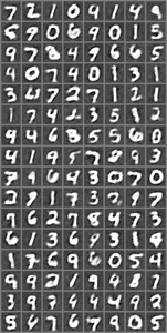
Reconstructed digits start to appear, but they are:
- blurry
- noisy
- low‑level shapes
- missing fine details
Interpretation
This shows the autoencoder beginning to:
- detect edges
- approximate shapes
- identify general digit structure
But the model is still far from accurate.
This image demonstrates early‑epoch learning.
Image 4 — Mid‑Training Reconstructions
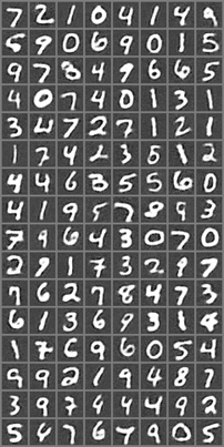
The digits are now:
- significantly clearer
- less noisy
- more distinguishable
- closer to the originals
Interpretation
This indicates:
- the encoder is learning to compress digit structure,
- the decoder is learning to reconstruct using that compressed representation,
- internal representations are stabilizing.
At this stage, reconstruction quality is visually acceptable.
Image 5 — Late‑Training / Final Reconstructions
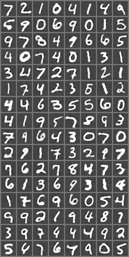
These reconstructions are:
- very close to the original images
- sharp
- clean
- high fidelity
Interpretation
This is the end of training reconstruction performance:
- Most digits match their originals almost exactly
- Stroke width, shape, and intensity are well preserved
- Noise is minimal
- The model generalizes well across a variety of digit shapes
Embeddings Visual Analysis
The autoencoder produces 64‑dimensional embeddings for each MNIST digit. To understand the structure of this latent space, we generated several visualizations:
PCA (Principal Component Analysis)
t‑SNE (t‑Distributed Stochastic Neighbor Embedding)
Statistical Summary Table
Each one reveals different properties of the internal representations learned by the model.
1. PCA Visualization — Global Structure of the Latent Space
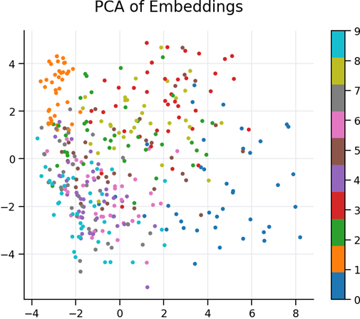
Figure: PCA 2D Projection of Embeddings
This PCA plot shows a two‑dimensional linear projection of all 64‑dimensional embeddings.
Key observations:
- Digits form distinguishable clusters, even after linear compression into only two dimensions.
- The clusters are not completely separated, which is expected, because PCA preserves global variance but not local relationships.
- The spread of points suggests that the embeddings capture rich variability between digit classes.
- Overlaps indicate that some digits share structural similarities (e.g., 1 vs 7, 3 vs 5), which is common in handwritten MNIST patterns.
Conclusion
PCA confirms that the autoencoder learned a meaningful latent representation, where digits are globally organized according to visual similarity.
- t‑SNE Visualization — Local Structure and Non‑Linear Relationships
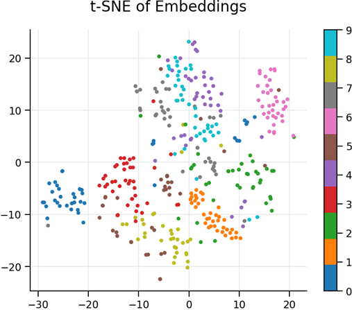
Figure: t‑SNE 2D Projection of Embeddings
The t‑SNE visualization provides a non‑linear dimensionality reduction, capturing local relationships more effectively.
Key observations:
- The digit classes form very compact and well‑defined clusters, much more separated than in PCA.
- t‑SNE reveals fine‑grained structure: digits with similar shapes remain close but still form distinct groups.
- Some digits (such as 0, 1, 6, 9) create extremely tight clusters, showing strong consistency in how the encoder represents them.
- The clear separation indicates that the latent features are highly discriminative, even though the model was trained only for reconstruction, not classification.
Conclusion
t‑SNE demonstrates that the autoencoder’s latent space exhibits strong internal organization, capturing digit identity naturally and non‑linearly.
Advanced Embeddings Analysis – Full Visual Set
The autoencoder embeddings are 64‑dimensional vectors. The following advanced plots allow us to understand:
- how dimensions relate to each other
- how classes cluster in latent space
- how the encoder distributes information
- PCA 3D — Global Linear Structure in 3 Dimensions
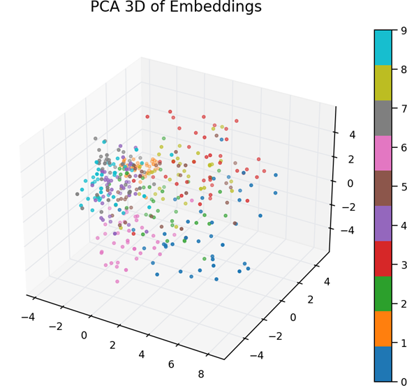
This 3D PCA projection provides a more expressive view than the 2D PCA:
- Digit clusters begin to separate more clearly in 3 dimensions.
- PCA continues to capture global variance, but still provides meaningful grouping.
- Similar digits (like 3, 5, 8) appear closer together, reflecting structural similarity.
- Distinct digits (like 0, 1, 7) spread out more clearly in space.
Conclusion:
The encoder distributes class‑specific information along different principal directions, indicating good latent structure.
- t‑SNE 3D — Non‑Linear Manifold Visualization
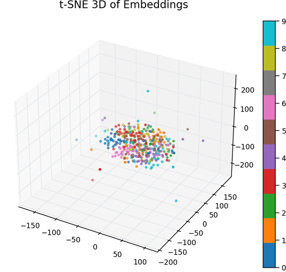
t‑SNE 3D reveals highly detailed and non‑linear structure that PCA cannot capture:
- Digit classes form dense, tightly‑packed clusters.
- Cluster boundaries are much sharper than PCA, showing that the embeddings contain strong class separation.
- Digits with similar shapes still appear near each other (e.g., 4 and 9).
Conclusion:
The encoder’s learned manifold has clear, non‑linear separability between digit classes.
This is strong evidence that the learned embeddings are highly expressive.
- Correlation Heatmap — Relationships Between Embedding Dimensions
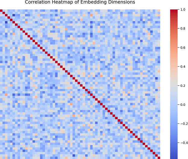
This heatmap shows pairwise correlations between all 64 latent dimensions:
- The mostly random pattern means the dimensions are not redundant.
- Some diagonal blocks hint at small subsets of dimensions capturing similar features.
- No strong linear dependencies are present — this is desirable, because it means the model is efficiently using many independent directions to encode information.
Conclusion:
The latent space is well‑decorrelated, meaning the autoencoder distributes information efficiently across dimensions.
4. Histogram Grid — Distribution of Each Latent Dimension
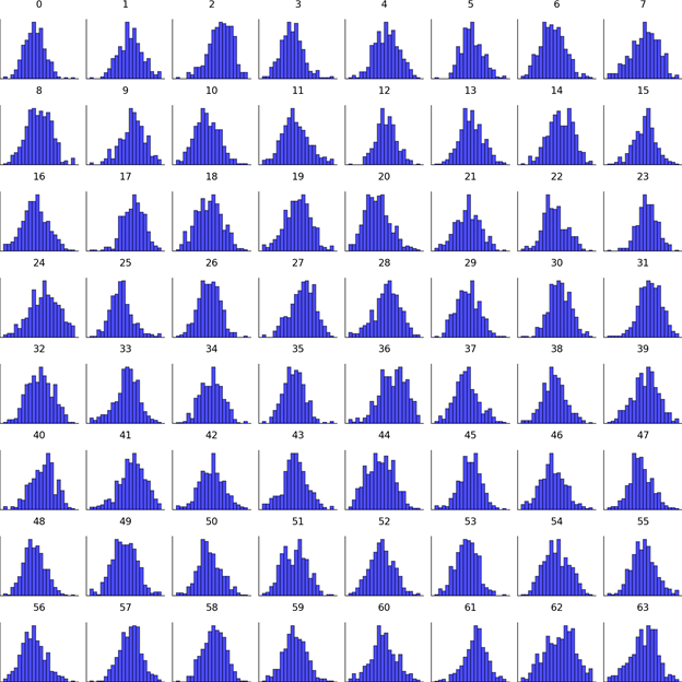
This grid shows a histogram for each of the 64 embedding components:
- Most dimensions follow smooth, centered distributions, typically around 0.
- Some dimensions have wider ranges, indicating they capture high‑variance features.
- No dimension collapses to a constant value — meaning no “dead neurons” exist in the latent vector.
- Some distributions show symmetry, others light skewness — typical of real image embeddings.
Conclusion:
The encoder uses all 64 latent dimensions actively.
This diversity improves reconstruction and cluster separation.
The autoencoder has learned a rich and well‑structured latent space:
- PCA (2D & 3D) : shows global organization
- t‑SNE (2D & 3D) : shows clear class clustering
- Heatmap : reveals independence across dimensions
- Histograms : prove active and diverse latent units
- Stats Table : confirms numerical stability and balance
 @Yolanda Muriel
