1948 – Bag-of-Words & Distributional Hypothesis
- Bag-of-Words (BoW):
Text is represented as an unordered collection of words, ignoring grammar and word order. Only word frequency matters. - Distributional Hypothesis:
“A word is characterized by the company it keeps.”
This idea states that words with similar meanings tend to appear in similar contexts.

© Image. Rahul Sharma NLP: Bag of Words
1954 – N-gram Models
- N-gram Model:
Predicts the next word in a sequence based on the previous n − 1 words. - This is a statistical approach that captures short-term word dependencies but struggles with long-term context.
1986 – Neural Probabilistic Language Models
- These models introduce neural networks to language modeling.
- Words are represented as continuous vectors (embeddings), allowing the model to learn similarities between words.
- This was a key step toward modern deep learning in NLP.
2003 – Distributed Representation
- Words or concepts are represented as patterns of activation across many dimensions rather than single symbols.
- This idea made it possible to capture semantic meaning more effectively and efficiently.
2013 – Word2Vec
- Word2Vec provides a simple and efficient way to learn word embeddings.
- Words with similar meanings have similar vector representations.
- It became widely used as a foundation for many NLP models.
2018 – Pre-trained Language Models
Large pre-trained models (such as BERT, GPT, etc.).
Key characteristics:
- Contextual word representations (word meaning changes depending on context)
- Pre-training + fine-tuning pipeline
- Use of large datasets and deeper neural networks
- These models significantly improved performance across many NLP ta
N-gram Models
When we want to predict the next word in a sentence, the most correct way would be to look at all the previous words.
For example, to predict word k, we would use: all words from the beginning of the sentence up to word k − 1.
This probability is written as: p(wₖ | w₁, w₂, …, wₖ₋₁)
The problem
- Using the entire history of words is very difficult.
- For long sentences, there are too many possible word combinations.
- It requires huge amounts of data and computation.
The Markov Assumption
To make the problem easier, we use the Markov assumption.
The idea is simple: The next word depends only on the last few words, not on the whole sentence.
So instead of using all previous words, we only use the last N words.
This approximation is written as:
p(wₖ | w₁:k−1) ≈ p(wₖ | wₖ−N+1 : k−1)
- N is the number of previous words we look at.
- N defines the order of the n‑gram model.
Examples:
- Unigram (N = 1): no context (each word is independent)
- Bigram (N = 2): depends on the previous 1 word
- Trigram (N = 3): depends on the previous 2 words
Example
Sentence:
«I want to drink coffee»
If we use a bigram model:
- To predict “coffee”, we only look at “drink”
- We ignore earlier words like “I want to”
Sequence Modeling Using RNNs
The goal of an RNN language model is to: Predict the next word using the previous words in a sequence.
Example sentence:
“the students opened their ___”
The model tries to predict the next word, such as “books” or “laptops”.
Computers cannot understand words directly, so:
- Each word is first converted into a one‑hot vector (a vector with zeros and one 1).
- This vector is then converted into a word embedding (a dense numerical vector).
This is done using an embedding matrix E:
e(t) = E · x(t)
Word embeddings store the meaning of words as numbers.
Hidden states (memory of the model)
The RNN has a hidden state, which works like memory.
At each time step:
The model takes:
- the current word embedding
- the previous hidden state
- It combines them to produce a new hidden state
Formula:
h(t) = σ(Wₕ h(t−1) + Wₑ e(t) + b₁)
The hidden state remembers information from previous words.
The same weights are used at every step → weight sharing.
Predicting the next word
The hidden state is then used to predict the next word:
ŷ(t) = softmax(U h(t) + b₂)
- Softmax produces a probability distribution over all words in the vocabulary.
- The word with the highest probability is the prediction.
Example:
- “books” high probability
- “laptops” lower probability
Why RNNs are powerful
- They process words one by one
- They keep information across time
- They do not use a fixed window like n‑grams
- They work with long sequences
- The input sentence can be much longer than in n‑gram models.
Key idea
An RNN reads a sentence word by word, keeps a memory of past words using hidden states, and uses that memory to predict the next word.
Self‑Supervised Pretraining
Self‑supervised pretraining is a way to train a language model using a lot of text without human labels.
Models like BERT learn language by reading massive text collections and creating their own learning signals.
Large‑Scale Text Data
- The model is trained on huge amounts of text, such as:
- Wikipedia
- Books
- These texts contain billions of words.
- The data is unlabeled, meaning no human says what the correct answer is.
This allows the model to learn grammar, meaning, and general knowledge from raw text.
Corpus Processing
Before training:
- The text is cleaned and split into smaller pieces.
- Special tokens are added:
- [CLS] used to represent the whole sentence
- [SEP] used to separate sentences
This helps the model understand sentence structure.
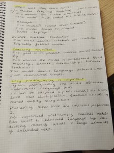
What “Self‑Supervised” Means
Self‑supervised learning means:
- The data itself creates the labels.
- No manual annotation is required.
BERT uses two main tasks:
a) Masked Language Modeling (MLM)
- Some words in a sentence are hidden (masked).
- The model must predict the missing words.
Example:
“The students opened their [MASK]”
The model learns to predict:
- “books”
- “laptops”
b) Next Sentence Prediction (NSP)
- The model learns whether one sentence logically follows another.
Training Objective
- The goal is to predict masked words correctly.
- This trains the model to understand:
- Word meaning
- Context
- Relationships between sentences
The model learns language patterns, not just memorized words.
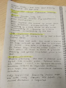
Why Pretraining Is Important
After pretraining:
- The model already understands language well
- It can be adapted (fine‑tuned) to tasks like:
- Text classification
- Question answering
- Named entity recognition
Pretraining saves time and improves performance.
Self‑supervised pretraining teaches models like BERT to understand language by predicting missing words in large amounts of unlabeled text.
Decoder‑Only Model: The GPT Model (Easy Explanation)
GPT is a decoder‑only Transformer model used to generate text.
What does GPT do?
GPT generates text by predicting the next word one word at a time.
- It reads text from left to right
- Each new word is predicted using all previous words
Example input:
“robot must obey …”
GPT predicts the next word:
“orders”
This is called next‑word prediction.
Why is GPT called “decoder‑only”?
A Transformer normally has:
- an encoder
- a decoder
GPT uses only the decoder part.
This decoder:
- looks at previous words
- predicts the next word
- does not need an encoder
This design is ideal for text generation.
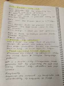
How does the decoder work?
GPT is made of multiple decoder blocks stacked together.
Each decoder block contains two main parts:
a) Masked Self‑Attention
- The model can only look at previous words
- It cannot see future words
- This keeps prediction honest (no cheating)
This is why it works left‑to‑right.
b) Feed‑Forward Neural Network
- Processes the output of attention
- Helps the model learn complex language patterns
Improves understanding and prediction quality.
Masked Attention
The mask ensures:
- Word 3 can only see words 1 and 2
- Word 4 can see words 1, 2, and 3
This makes GPT autoregressive:
- It generates text step by step
Large context window
- The model can see up to 4000 tokens
- The more context it has, the better predictions it makes
That’s why GPT can write long, coherent text.
GPT is a decoder‑only Transformer that generates text by predicting the next word using masked self‑attention and past context.
Greedy Sampling
Greedy sampling is a simple method used by language models (like GPT) to generate text.
The idea is very straightforward:
At each step, the model always chooses the word with the highest probability.
How Greedy Sampling Works
When the model wants to generate a sentence, it works one word at a time.
At each position:
- The model calculates the probability of every possible next word
- It selects the word with the highest probability
- That word is added to the sentence
- The process repeats for the next word
There is no randomness involved.
Example from the Image
Given the sentence start:
“Paris is …”
Step by step prediction:
Position 1
- “of” 0.337 (highest)
- “that” 0.153
- “where” 0.094
Selected word: “of”
Position 2
- “the” 0.218
- “history” 0.03
- “love” 0.02
Selected word: “the”
Position 3
- “future” 0.024
- “world” 0.018
- “city” 0.016
Selected word: “future”
Position 4
- “.” 0.324
Sentence ends
Final generated text:
“Paris is of the future.”
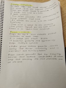
Key Characteristics of Greedy Sampling
Always chooses the most probable word
Very fast and deterministic
Same input : same output every time
Limitations of Greedy Sampling
Can produce boring or repetitive text
Can miss better sentences that require choosing a less probable word early
Not very creative
Example problem:
- Choosing a safe word too early may block a better sentence later
Greedy sampling generates text by always choosing the most likely next word, without randomness.
Beam Search
Beam search is a method used by language models (like GPT) to generate better sentences than greedy sampling.
Instead of keeping only one best word choice, beam search keeps several good sentence options at the same time.
Key Idea
Beam search keeps the top k most probable partial sentences at each step.
- k is called the beam width
- It balances quality and efficiency
How Beam Search Works
Assume the model starts with:
“Paris is the city …”
Step 1 (First word)
The model predicts several possible next words:
- «of»
- «is»
- «has»
Instead of choosing only one: Beam search keeps the best k options
Step 2 (Next word)
For each saved sentence, the model:
- Predicts the next word
- Calculates the total probability of the whole sentence
- Keeps only the top k best sequences
Worse options are discarded
Better options continue
Step 3 (Repeat)
This process continues:
- Expanding each candidate sentence
- Keeping only the best k sentences at each step
At the end: The sentence with the highest overall probability is chosen.
Example Outcome
Instead of greedy output:
“Paris is of the future.”
Beam search may output:
“Paris is the city of culture.”
More fluent
More meaningful
Greedy vs Beam Search
| Method | Keeps Multiple Options? | Result Quality |
|---|---|---|
| Greedy Sampling | No | Can be short or awkward |
| Beam Search | Yes | More coherent sentences |
Advantages of Beam Search
Better global sentence quality
Avoids early bad choices
Commonly used in translation and summarization
Disadvantages
Slower than greedy decoding
Can generate less diverse text
Large beam width = more computation
Beam search generates text by keeping several best sentence candidates at each step and choosing the most probable one at the end.
Bonus
I recommend you always write down your ideas on paper, in order that AI do not write them.
 @Yolanda Muriel
